Packet Ray Tracing
with the
ARM NEON Architecture
keywords
Packet Ray Tracing, ARM, NEON, SIMDARM Sweden AB \supervisorJohan Grönqvist, Johan.Gronqvist@arm.com \examinerMichael Doggett, mike@cs.lth.se \dedicationThis work is dedicated to you, Eliza. Thank you for all the wonderful years you have given us. \theabstractThe ray tracing algorithm has long been used to create near photorealistic images and even simple ray tracers can simulate effects such as shadows, reflections and refractions where other methods struggle. Today, the state-of-the-art CPU ray tracers are typically those that are able to efficiently leverage data-level parallelism at the instruction level by using SIMD extensions to allow the processor to trace multiple rays simultaneously, rather than one at a time. Within the ARM processor, the SIMD architecture is known as NEON and it is used to speed up data-parallel applications such as multimedia decoding and computer graphics. Thus, in this thesis we have investigated the implementation and performance of a ray tracer that utilizes the NEON architecture to trace packets of rays similar to modern ray tracing frameworks. To determine the efficiency of it we also developed a single-ray tracer as a reference and compared them in regard to both runtime and power consumption. In the end, we found that the optimized ray tracer scales better and performs around 150 – 300% better than the reference single-ray tracer. \makefrontmatter
Chapter 1 Introduction
1.1 Outline
Ray tracing has been used for a long time to generate images that closely mimic what happens in nature and can thus create almost photorealistic images. This imaging process is however often very slow when compared to the rasterization algorithm and has thus almost exclusively been used in offline rendering pipelines.
Despite the recent trend of using GPU:s to accelerate the computations, the most common compute unit in ray tracing pipelines is still the CPU. There are many reasons for this e.g., The ease of programming, GPU memory bottlenecks or high price per unit. Among the CPU s the x86 architecture is currently the dominant processor architecture, thus performance-oriented applications such as ray tracers are almost always optimized for this architecture.
One of the more powerful optimizations provided by modern processors are the so called SIMD extensions. These extensions allow users to issue special instructions that will operate on multiple values at once, greatly increasing performance if used correctly.
Modern designs of the ARM processor now includes SIMD extensions. Still, the ARM architecture is generally not regarded as a powerful one but its performance has greatly increased with the introduction of the Cortex-series CPUs. The availability of these chips has also improved; many development boards such as the Pandaboard [24] or smaller laptops such as the Samsung Chromebook [27] are readily available and cheap for the developers.
These platforms were not originally intended for heavy computing but the modern ARM processors inside many of them are often very powerful and many also include the ARM counterpart to SSE: NEON [22]. With this extension, ARM processors can be heavily optimized for a wide variety of applications including video decoding, image processing and computer graphics.
While Ray tracing is a type of computer graphics, no public effort have yet been made to create a ray tracer optimized for the ARM architecture. With this thesis we attempt to create such a ray tracer and evaluate its possible advantages.
We will begin with introducing the reader to the background of both ray tracing and SIMD accelerated computing here in chapter 1. Following in chapter 2, we describe some implementation specific details of the ray tracer created during the project. In chapter 3, we describe our methods used to evaluate the runtime-performance and power-consumption of the ray tracer on a selection of ARM platforms. Our expectations and hypotheses are then outlined in chapter 4 and the actual results are compiled in chapter 5. A discussion of the results follows in chapter 6 and our conclusions and future work are outlined in chapter 7. In addition, some extra notes regarding the ARM hardware design and the differences between SSE and Neon can be found in the appendices A - B.
1.2 Background
1.2.1 Ray Tracing
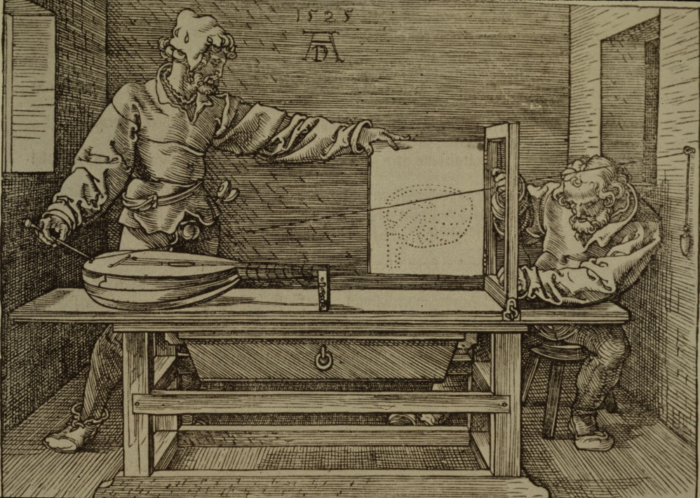
Ray tracing is not a new method of rendering graphics. It is even arguably the oldest method of generating accurate perspective-correct images. Historical records show us that mechanical analogues to ray tracing were used as far back as in 1525, as seen in the woodcut in figure 1.1.
One of the earliest examples of using computers to render images with ray tracing techniques is with the so called ray casting algorithm, originally presented by Arthur Appel in 1968 [1]. The idea behind this algorithm is to trace rays from a virtual camera (with at least one ray for each pixel) into the scene and compute the color of the object closest to it. This simple algorithm could then be used to apply simple shading to the objects, but lacked many of the features found in ray tracers today such as shadows, reflections and refractions.
These limitations were however fixed by Turner Whitted [34] who introduced the first true ray tracing algorithm which is today commonly referred to as Whitted style ray tracing algorithm. Whitted’s method works similarly to the ray casting algorithm but the major difference is that it works recursively. Rays are still traced from the camera but at the intersection point, new rays are generated in the reflecting or transmitting directions. This addition will give us perfect reflections and refractions but to also get the shadows, some more work is needed. At each intersection point we also trace new rays toward each light source in the scene. If that ray hits the light source, or more accurately; if it does not hit anything in the scene, the point should be shaded normally. Otherwise it is in shadow and should not be shaded.
Distributed Ray Tracing
Whitted’s extension added many pleasing aestethic effects, but they were in a sense too perfect. Since only hard shadows and perfect specular effects are generated, many of the ‘softer’ effects such as glossy reflections or soft shadows cannot be simulated with Whitted’s approach.
One way to add these softer effects is to attach distributions to each effect, as suggested by Cook with his Distributed Ray Tracing algorithm [7]. This way we can get soft shadows by generating a number of rays in the general direction of the light source and then average the resulting shading over the rays that actually hit the source. Repeating this over several points can thus create accurate penumbras for the shadows. Similarly, glossy reflections and translucency can be simulated by sampling distributions of rays in the reflecting and transmitting directions respectively.
Path Tracing and the Rendering Equation
The additions provided by Cook takes us a long way, easily achieving effects that are difficult to re-create in a rasterization pipeline.
Cook’s approach suffers from a very drastic drawback however: at each point we must generate a number of rays toward the light and in the specular directions. This means that after only a few recursive steps, we have generated so many rays that the image will take a very long time to render. In addition, effects which require slightly more recursive steps can be missed entirely, and effects such as indirect lighting, color bleeding and caustics are not easily integrated in Cook’s algorithm. Thus, in order to improve both the quality of the images and possibly improve the rendering speed, a more complicated model is needed.
One such model is provided by the so called Rendering Equation shown in the equation below and was originally presented by Kajiya [17]. By approximating the solution to this equation, we can create increasingly better and more photorealistic images. It should be noted however that the equation shown here is just one variant of the rendering equation, there are several more complex ones that can simulate additional phenomena. E.g. wavelength information can be added to account for diffraction, fluorescence and scattering.
| where | |||
| x | |||
| n | |||
Over the years, several algorithms have been developed to approximate this equation. When Kajiya presented it however, he also presented the so called Path Tracing algorithm he used to approximate it. This algorithm is a Monte Carlo method; it uses random values in an input domain to approximate the result, which in this case is the integral shown in the equation above.
The general idea behind the algorithm is to re-use Whitted’s ray tracing algorithm. Instead of tracing the reflected and refracted directions however, we randomly decide if we should trace them, or a completly random direction using pseudo-random numbers. Furthermore, at non-specular points, we still generate a new ray in a random direction on the hemisphere centered around the normal of the intersection point. Doing this in several steps creates a single path for the ray, giving the algorithm its name. In order for this algorithm to generate truly realistic images however, often several thousands of ray paths must be traced per output pixel in the image.
Acceleration Data Structures
Regardless of the ray tracing algorithms used, each time we generate a ray we must perform intersection tests with all the primitives in the scene to determine if it will in fact hit anything and if it does, which of them is the closest one. With this naive approach we easily see that the complexity of the algorithms are proportional to:
It is however possible to drastically reduce the number of tests that are required, to around the order of
by using special data structures that order the scene data prior to the rendering. There are a large variety of ways this can be done but some of the more popular algorithms used are Uniform Grids, Binary Space Partitioning Trees (BSP-trees), and Bounding Volume Hierarchies (BVH). Detailed explanations and implementations of all of these algorithms can be found in e.g., [25].
Each of these work in different ways and have potential advantages or disadvantages depending on the given scene. In general terms, all of them attempt to subdivide the scene so that each time we trace a ray, we only have to query a subset of all primitives.
1.2.2 Single Instruction Multiple Data
In Flynn’s taxonomy [12], SIMD is a class of parallel processing computer architecture. Computers processing vectors of data has been around for a long time. Many of the first supercomputers, such as the CDC STAR-100, could process vectors of data with a single instruction. These kinds of architectures are regarded as different ones compared to SIMD architectures, since these vectors are processed one word at a time whereas SIMD process all elements simultaneously, as illustrated in 1.2.
The SIMD architectures seen today grew out of a demand of real-time processing in the desktop-computer market. To meet this new requirement, processor vendors began to implement instruction set extensions to their processors to allow users to process vector elements in a SIMD fashion.
The first available SIMD instruction set extension was the UltraSparc Visual Instruction Set [18], with other vendors such as MIPS and Intel quickly following suit with the MIPS Digital Media eXtension and MMX respectively.
Some time later, Motorola introduced AltiVec as a much more powerful SIMD processing extension for the PowerPC architecture. Intel responded to this by developing the Streaming SIMD Extensions, which along with its successor, the Advanced Vector Extensions, has become the most widely available and used SIMD extensions to this date and compiler intrinsics are available from several of the most important compiler developers. [13, 31, 19]. ARM processors are however also becoming increasingly common and now also offer a SIMD extension of their own, known as NEON111The official name for NEON is actually Advanced SIMD Extension but in the interest of brevity and readability, we will reduce the name to Neon instead, with a single capital letter., offering much the same functionality as SSE.
1.3 Related Work
All rays in a ray tracer are inherently computationally independent from one another, meaning that the ray tracers are amenable to most kinds of parallelization. It is thus very easy to extend the ray tracing algorithms to multicore architectures and even to multi-program systems.
Rays that travel in roughly the same direction often take the same way through the acceleration data structure and often hit the same or adjacent primitives in the scene. By grouping adjacent rays into packets and tracing them simultaneously, it might be possible to improve the performance. Ingo Wald showed in his thesis [33] that such a grouping greatly improved the ray casting and ray tracing performance when using SSE intrinsics and carefully cache aligned structures.
Wald’s work has lead to further research into ray tracing algorithms using packets of rays rather than single ones. Typically, this kind of ray tracing algorithms are called packet ray tracing, or simply packet tracing. So far however, almost all research has been done using SIMD as a general term, but in practice, they are often only implemented with SSE in mind, despite having several competing technologies available, such as Neon.
Furthermore, there have not been many attempts to estimate the performance of modern ARM processors with the Neon extension. Two comprehensive comparisons with a wide variety of synthetic benchmarks do however give a clue of how well they perform, in particular they show us that these platforms might be well suited for ray-tracing [23, 26].
There has also been some study on the comparative performance between several highly optimized ray tracing frameworks [30]. These comparisons were however performed on Intel CPUs and Nvidia GPUs, using software technologies and frameworks unavailable in ARM CPUs. Thus it is difficult to use these results as a comparison.
1.4 Problem Formulation
So far, almost all research on ray tracing has been performed on GPUs, Intel CPUs, or a combination of these. It is however worth noting that Intel:s x86 architecture is far from the only CPU architecture. With the introduction of the Neon SIMD architecture in modern ARM CPUs, it is of interest to see if it can be used to create high-performing ray tracers, similar to how frameworks such as Embree [35] and RTRT/OpenRT [33] are constructed.
We will investigate how such a system could be constructed and how the Neon architecture could be utilized to improve the ray tracing performance by exploiting the inherent coherency of primary, shadow and first specular rays. Since we are primarily interested in the direct ray tracing performance, we will limit ourselves to a Whitted style ray tracer and only consider simple materials and light sources. Moreover, exotic features such as texturing and instancing are outside the scope of this project.
This ray tracing application will be developed with the ISO C++11 standard [15] but in order to efficiently access the Neon architecture we will also make use of compiler specific extensions. The ambition is follow the standards as closely as possible to make the framework portable and potentially extendable to other SIMD architectures.
Finally, we will attempt to estimate the energy consumption of the application and, when possible, both the runtime and energy consumption will be compared with prior research on x86 CPUs and GPUs.
Chapter 2 Implementation
The Neon architecture has previously, and successfully, been integrated in the software libraries such as ffmpeg [11] and Eigen [10] where it has provided various speedups. In, e.g., ffmpeg the performance increase with Neon was around a factor of 2 for one platform [29].
In order to make sure our ray tracing application performs as well as possible, we carefully design it with performance in mind. Since there has been little to no work on creating a Neon accelerated ray tracer in the past, we will develop parts of it based on how other SIMD frameworks such as Embree [35] and RTRT/OpenRT [33] have been developed.
The ray tracing system itself is made up of two distinct parts: the ray tracer itself and a SIMD Mathematics Library that is configurable at compile time. In order to make the ray tracer as portable as possible, only the ARM Neon extensions are used beyond the normal capabilities of the compiler. The system also makes full use of the ISO C++11 standard to access the cross-platform memory alignment and threading models and thus require a rather modern compiler, such as GCC-4.8 [13] or LLVM-3.4 [19].
2.1 The SIMD Library
The mathematics library provides the basic vector operation tools used throughout the system, including optimized vector and matrices types. Among the vector types, three basic vectors are used frequently throughout the system:
- neon4f
-
A vector with four 32-bit floating point values.
- neon4i
-
A vector with four 32-bit signed integer values.
- neon4b
-
A vector with four 32-bit unsigned integer values interpreted as a boolean vector mask.
These types are wrapper classes around the data types provided by the Neon extension. These classes also overload all relevant arithmetic operations as well as providing additional functionality needed for vector calculations.
The ray tracer is designed to be able to switch between the SIMD mathematics library and a second, strictly floating point library, implementing the same functionality with arrays of values rather than SIMD data types. This abstraction is done to easily compare the performance with a non-Neon-enabled ray tracer. This switch is performed at configuration time, so no run-time performance is lost through the abstraction. This also makes the system portable to platforms and compilers without Neon support, albeit with potential performance reductions. It should however be noted that even in the non-Neon-enabled ray-tracer, Neon may still be used by the compiler to try to optimize the application.
In order to implement the grouping of adjacent rays into packets [33], the library also contains vector types with arrays of three basic vectors. Where each vectors represents a single dimension for 4 separate vectors; a layout typically called Structure of Arrays. This layout is illustrated in figure 2.1. With these vector types, the normalization, dot-product and cross-product operations are very cheap to perform, since no expensive horizontal movement across the vector is required.
⬇ struct Vec4x3 { neon4f x; neon4f y; neon4f z; };
2.1.1 Memory Alignment
Compared to conventional programs, SIMD enabled algorithms and data structures often have very strict memory alignment requirements. The Neon architecture, e.g., can allow unaligned access by setting some bits in a system register, but the unaligned access will still be slower than a properly aligned accesses [4, A3-108].
Thus, in order to use our Neon vector types, it is important to ensure their memory alignment on both the stack and the heap. The ISO C++11 standard introduced alignment specifiers that could be used to enforce an over-alignment of objects [15]. However, this specifier only applies to the stack alignment of objects and the standard does not specify how these over-aligned objects should be stored when stored on the heap.
To ensure that these objects are also properly aligned on the heap, we implemented custom memory allocation algorithms that exclusively allocate aligned memory.111The C++11 library function, align can handle this, but at the time of this writing, it is unimplemented in GCC-4.8, thus a custom one was implemented to make the system more portable. With these we could overload the member functions operator new and operator delete to ensure objects could be allocated directly on the heap. To also be able to use the C++ standard library containers, we implemented a custom allocator class for these containers.222Hopefully, these heap alignment issues should be fixed in a future revision of the C++ standard. [21]
2.2 The Neon Ray Tracer
The system is designed towards performance and is thus not as versatile in some regards compared to other ray tracing systems such as PBRT [25]. For instance, this ray tracer exclusively uses triangles as the basic primitive and only renders using Whitted style ray tracing.
2.2.1 Whitted Ray Tracing
The basic ray tracer design is based on the algorithm outlined by Turner Whitted [34]. Pseudocode of the algorithm used in our project can be be seen below in listing 1.
2.2.2 Acceleration Data Structure
Today, there are many data structures that can be used to accelerate the intersection testing in ray tracers. Some of the more common ones include the universal grid, Kd-tree and bounding volume hierarchy algorithms. While they all work differently, they share a common goal of reducing the number of primitives that have to be tested each time we trace a ray. For this project, we decided to use the bounding volume hierarchy, or BVH-algorithm, since it is a popular choice in many modern rendering pipelines.
To construct this structure, we begin with iterating over all primitives in the scene, creating a single axis aligned bounding box, or AABB that encapsulates all of them. This box is then recursively subdivided, until only a small number of primitives are stored in the final box. This way, a ray need only query a small number of bounding boxes and an even smaller number of primitives to determine if anything was actually hit.
Movement within an acceleration data structure is typically called traversal and this terminology will be used frequently later on.
2.2.3 Whitted Packet Tracing
In a regular ray tracer, at each intersection it is easy to compute which primitive was hit, what material said primitive has, what properties it has, which direction we should recurse toward if reflective, etc. Such decisions are much more complicated for a packet tracer, since at each intersection, more than one primitive might be hit. Even worse, the rays might hit different meshes or not hit anything at all! This causes the ray packet to have to traverse a considerably larger amount of BVH-nodes before it can exit, and for each node, all rays must be tested. These scenarios are illustrated in figure 2.2.
There are several ways to correct these scenarios. For instance, at each positive primitive intersection we can compute and store all data necessary for shading and generating secondary packets and mask away the results for the rays not hitting that particular primitive.
This works just fine for smaller scenes with few primitives and only a small number of effects to account for. It is however worth noting that this storing and masking of results occurs in one of the innermost loops of the ray tracer where we typically want to reduce the number of instructions as much as possible. Furthermore, when we start to scale the ray tracer with effects such as texturing, we have to compute additional data for that inside the loop as well. Thus, this approach will not scale very well and can quickly become a bottleneck.
A different approach solves these issues: After the intersection test, only compute and mask away the data necessary to return to the primitive after the traversal. Then afterwards, compute all necessary data needed for the shading and generation of secondary rays. This reduces the number of computations required in the inner loops and makes it easier to add more effects to the packet tracer later on with a minimal performance impact.
Despite these differences in the packet tracer, the actual packet tracing algorithm is almost the same as the single-ray one, as seen in listing 2. It also shows us a potential issue with packet tracing: When only a few rays in a packet intersects specular objects, a whole new ray packet must be generated and traced. For coherent rays, such as those generated by Whitted’s algorithm, this is usually not an issue, but must be handled to avoid artifacts.
2.2.4 Parallelization
Each ray or ray-packet in the renderer is computationally independent from one another. Only the scene data is shared between the rays, but the accesses are read-only, so no synchronization is required. It is however desirable for the same threads to access memory which are spatially close to potentially improve the number of cache hits.
To do this, we implement a simple image traversal scheme for the tracing threads. First, we make sure the image dimensions are rounded to even numbers, then we divide the image into tiles with a user specified size. Finally, each thread will atomically333This is the only synchronization required within this part of the ray tracer. select a tile-index, and trace all pixels, or packets inside the tile before requesting a new tile-index. This subdivision is shown in figure 2.3.
2.2.5 Runtime
The system executes four basic stages during each rendering, they are:
-
1.
Parsing
-
2.
Preparation
-
3.
Ray Tracing
-
4.
Output
We will describe each of these stages in greater detail in the following sections.
Parsing
When execution begins, the application first parses the user-input command-line options. One of these specifies a scene description file that will be parsed and all objects contained therein such as the cameras, lights and meshes are created and placed in the scene. Currently, the application supports some hard-coded, built-in scenes as well as a subset of the PBRT scene description format.444The full format specification is available here: http://www.pbrt.org/fileformat.php
Due to the limited amount of time and scope for the project, some of the features we removed from the PBRT format included: Instancing, complicated materials and light sources and texturing. Some non-triangle primitives used in the PBRT are also supported, they are however converted to triangles through tessellation rather than used as they are. Still, some scenes that use these unsupported features can be used, but will receive placeholders values when used.
Even with these limitations the PBRT format gives us access to a wide range of scenes, from rather simple ones such as single spheres and point-light, to relatively complicated ones, such as the YeahRight sculpture which can be seen later on in section 3.5.
Preparation
During the preparation stage, various computations are performed:
-
•
Point- and vector-data in meshes, cameras and lights are transformed to their final location or direction respectively.
-
•
The acceleration data-structure is constructed. In this project, the so called Bounding Volume Hierarchy is used as an accelerator [28, p.131].
-
•
Various values are cached to avoid costly re-computations.
Ray Tracing
In this stage the actual ray tracing is done. Looking closer at how this step works, we can break this particular step down some more:
-
1.
First, we generate either one ray per pixel for single-ray tracing, or a bundle of rays in a ray-packet from a 2x2 packet of pixels if we are packet tracing.
-
2.
Traverse the bounding volume hierarchy with the ray or ray-packet until we can conclude that either rays missed the scene, or that the closest hit points can be determined. At each positive primitive intersection, store only the data that is necessary to return to this particular primitive later, if the current one turns out to be the closest one.
-
3.
Once the closest primitive is found, compute the hit-point and normal directions, and optionally compute the transmitting or reflecting directions depending on the material the rays hit.
-
4.
Finally, shade the current pixel and optionally use the colors from additional rays from the reflecting and transmitting directions.
These steps are repeated for all pixels or 2x2 tiles of pixels, generating our ray traced image.
Output
Among the last things the application does is write the final image to disk in the PPM format555A description of this format is available at: http://netpbm.sourceforge.net/doc/ppm.html and write statistics generated from the rendering phase to standard output.
Chapter 3 Approach
Looking at some previous results of ray tracing on some ARM platforms, it does not seem to be possible to do it in real-time yet [23, 26]. Thus, we restrict the project to measure the performance for the generation of a single frame.
To evaluate this performance we will estimate the scalability, runtime performance and the energy consumption for each possible configuration of the ray tracer. These measurements will also be carried out on a few different hardware platforms as listed in section 3.1. Due to the varied construction of the platforms however, we must use different methods to estimate the power performance for each of them.
3.1 Test Platforms
The application will be evaluated on several different ARM based platforms, with the principal CPUs being the Cortex-A15 and Cortex-A9. A slightly more in-depth comparison between these processors and their respective features is included in appendix A.
The Cortex-A15 is estimated by ARM to perform roughly 50% better than the Cortex-A9 chip for the same core and frequency [16]. The A15 chip can however also operate at higher clock frequency, resulting in an even greater performance at the expense of the energy consumption. All this must be factored in when we make our assumptions regarding the expected performance.
Below we list the hardware platforms used for our measurements, including clock timings and cache sizes.
| Platform | Pandaboard Rev. A3 | Samsung Chromebook (XE303C12) |
|---|---|---|
| SoC | Texas Instrument OMAP 4430 | Samsung Exynos 5250 |
| CPUs | Cortex-A9 2@1.0 GHz | Cortex-A15 2@1.7 GHz. |
| L1 Cache | 32 KB instruction, 32 KB data | 32 KB instruction, 32 KB data |
| L2 Cache | 1 MB shared | 1 MB shared |
| Platform | CoreTile Express (V2P-CA9x4) | |
| SoC | ARM development reference | |
| CPUs | Cortex-A9 4@400 MHz | |
| L1 Cache | 32 KB instruction, 32 KB data | |
| L2 Cache | 512 KB shared |
3.2 Configurations
The performance of the ray tracer is estimated in four different configurations:
-
•
Scalar Single Ray Tracing
-
•
Scalar Packet Ray Tracing
-
•
Neon Single Ray Tracing
-
•
Neon Packet Ray Tracing
The Neon configuration activates the Neon extensions defined in the SIMD library and uses them to attempt to accelerate the application. In the scalar setup the vector libraries are replaced with the floating point equivalent, which perform the same operations as the SIMD instructions but executes them serially. The single ray tracer will also be used as the reference when comparing to the performance of the rest of the ray tracers.
3.3 Render Settings
In order to ensure consistent and comparable results between the different scenes and configurations, we will keep all rendering parameters fixed. That means that:
-
•
All frames are rendered at 1024x1024 pixels
-
•
Only a single sample is taken per pixel
-
•
A maximum of 3 recursive calls are allowed for reflection/refraction
-
•
The thread count is set to match the number of cores in the processor
3.4 Measurements
3.4.1 Scalability
It is well known that each ray is computationally independent from one another, and thus the ray tracer should scale linearly with the number of available compute units. We will test this on each platform by running our application with a varied number of threads up to the maximum number of cores available among the platforms. In the interest of brevity however, we will only include the results for a single scene.
3.4.2 Runtime Measurements
The performance of the platforms will be estimated in a number of ways. Internally, the ray tracer keeps track of some statistics, such as the time to render the frame or number of rays generated per second. Externally however, we use a variety of operating system tools and extra hardware to estimate the energy usage.
During runtime, the follow metrics are gathered inside the ray tracer:
-
•
Time to render the image
-
•
Time to build the bounding volume hierarchy
-
•
Generated primary rays per second
-
•
Generated shadow rays per second
-
•
Generated secondary rays per second
-
•
Bounding box Intersection tests per second
-
•
Triangle intersection tests per second
3.4.3 Power Measurements
To begin with, we have no physical access to the the CoreTile Express platform, so no power data will be obtained from it. For the remaining platforms, we will use different methods for each one of them. Before we gather any measurements we will compute a baseline energy consumption during idle for the platforms to reduce the impact of noise coming from various unrelated sources, such as the network chips. To further reduce such noise, all unrelated hardware is shutdown when physically possible. E.g. the screen on the Chromebook is powered down during all tests. Finally, to account for noise and input errors in the power data we will repeat the experiment a number of times to compute an average and confidence interval.
Measuring Power on the Pandaboard
For the Pandaboard, we will use an oscilloscope to measure the drawn current from the board directly. The oscilloscope we will be using is a Tektronix TDS3034. This oscilloscope can however only retain data for the last 100 seconds, which is not enough for some of the scenes we have chosen.
As a workaround, we will connect it to the Instrument Control Toolbox within Matlab and successively save the data until the ray tracer finishes executing. When it finishes, we can compute the energy consumption using the known constant V input voltage and the Power Rule (3.1). Finally, we use the trapezoidal rule to approximate the total amount of energy used to run the application.
To also retrieve the energy consumed to rendered the actual frame, we will repeat the computations noted above but change the start time and end time to account for time spent parsing, building the BVH before rendering and deallocating resources afterwards.
| (3.1) |
Measuring Power on the Chromebook
The modern Linux distribution all include synthetic file systems that allow applications to easily access kernel information. Some such information include current power management information and settings. This means that e.g. laptops can use these ‘files’ to access battery data.
In our case, we can access battery information for the Chromebook from various files in the /sys/class/power_supply/sbs-4-000b directory. By regularly polling these files, we can estimate the present voltage, current, charge, etc. from the battery. With these, we can once again use the Power Rule (3.1) to compute the power, and the trapezoidal rule to estimate the energy consumption.
3.5 Test Scenes
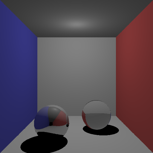
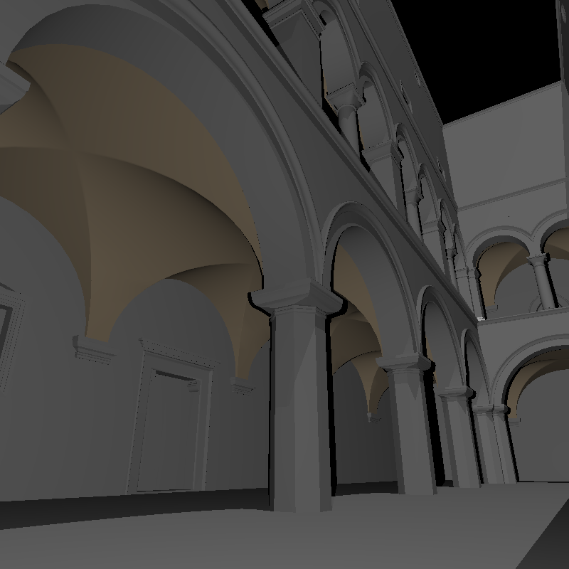
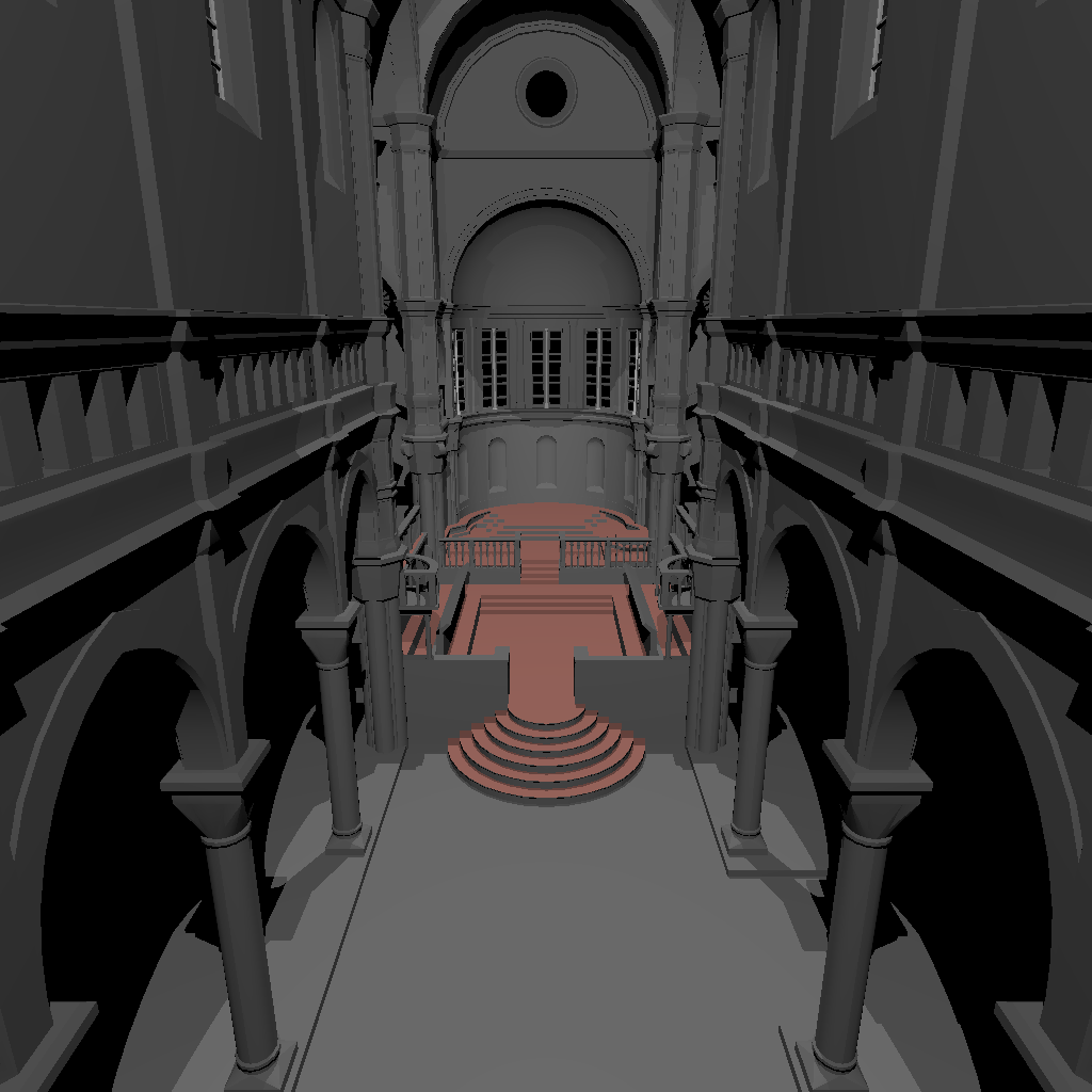
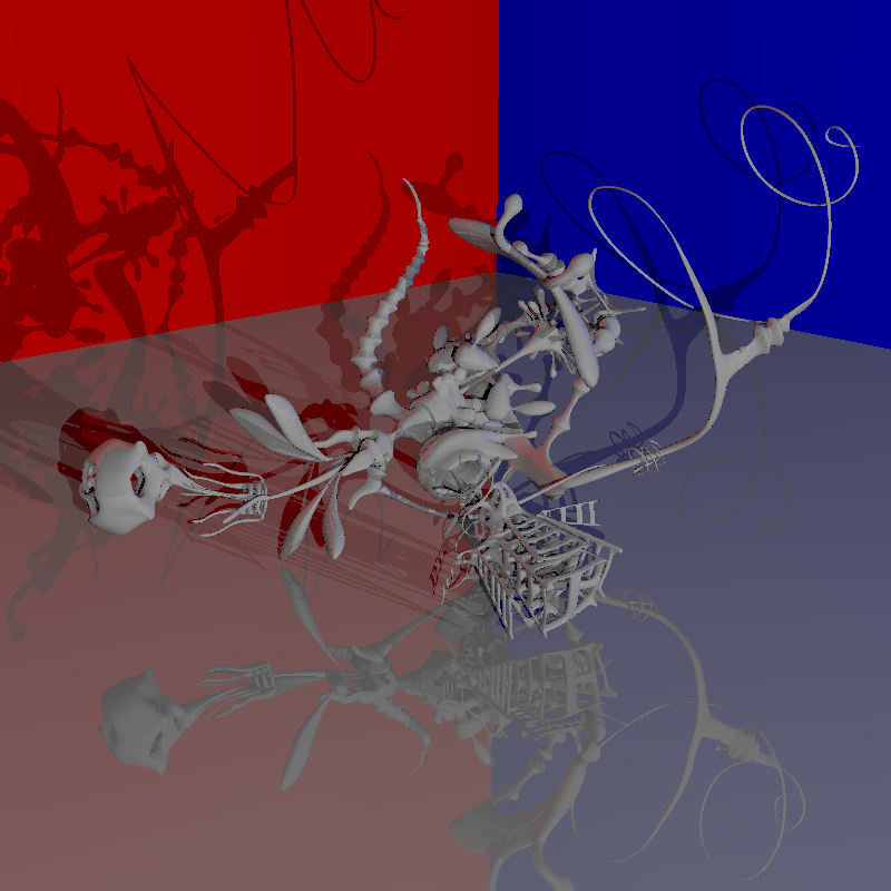
A variety of scenes are used to estimate the performance of the ray tracer, each with a triangle count varying between to around triangles. An exact number of triangles for each scene is shown in Figure 3.1.
-
•
The Cornell box model is available at:
http://www.graphics.cornell.edu/online/box/data.html -
•
The YeahRight model is available at:
http://www.cs.columbia.edu/˜keenan/Projects/ModelRepository/
Chapter 4 Hypothesis
Considering some previous benchmarks [23], the Chromebook seems to have a floating point performance of around 3-5 times higher than that of the Pandaboard. The same test suite also contains results from the smallpt-benchmark111http://www.kevinbeason.com/smallpt/, where the Chromebook perform around 3 times better than the Pandaboard, giving us an estimate of how well ray tracing might be on these platform. If we account for the clock speed being around 70% higher on the Chromebook however, the clock for clock performance is reduced to around 1.5–2 times instead.
Based on these results, we hypothesize that the Cortex-A15 will render scenes roughly 3 – 5 as fast as the Cortex-A9 when including the clock rates. All other runtime metrics are expected to follow this with some variations based on the materials in the scene. Moreover, we expect all variants of the ray tracer to scale almost linearly with the number of available processing cores.
Based on Wald’s results [33, p.122], we also expect the packet-ray-tracers to perform around 2-3 times better than the equivalent single-ray-tracers for all the scenes we have chosen to test on. Among all configurations, we believe that the Neon accelerated packet-tracer should be the fastest one.
Finally, we believe that the energy consumption should be rather small, and should scale about as well as the runtime performance.
Chapter 5 Results
All results we have gathered during this project are compiled in this chapter. Similarly to the earlier chapters, the results are divided into 3 sections:
-
•
Runtime Performance
-
•
Scalability
-
•
Power Performance
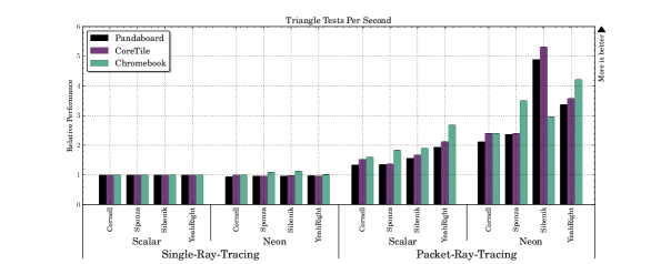
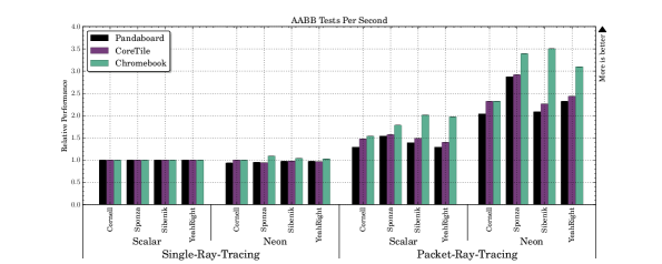
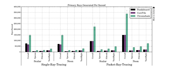
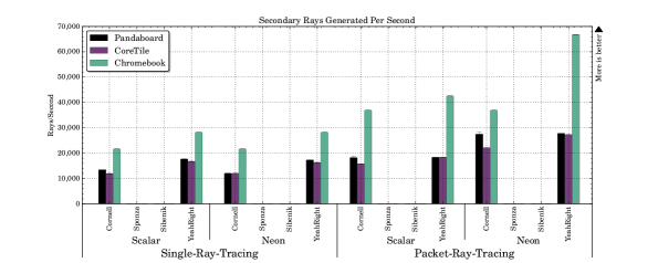
It should be noted that the packet tracer algorithms generate rays and perform tests on groups of 4 rays at a time. Thus, each time a packet tracer is executed the corresponding tally is increased by 4 rather than 1, even if some of the rays were invalid inside that particular packet.
The bar graphs shown here represent the average over a number of runs and the black caps on the top of each bar represent the confidence interval. This cap is however often very small and might not be seen in many of the plots.
For a more thorough discussion of the results in this chapter, see the discussion chapter (6). Some additional data collected during the course of this project can be found in appendix C.
5.1 Runtime Performance
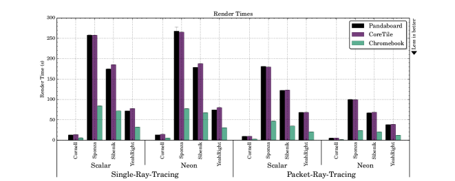
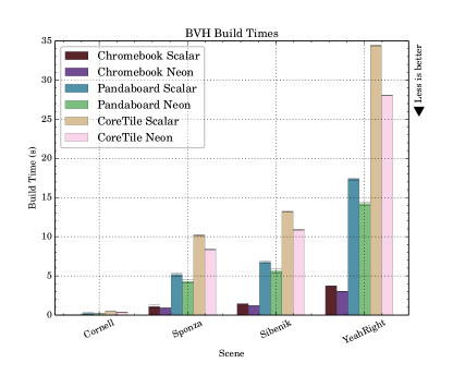
The various runtime measurements are summarized in the figures below.
5.1.1 Relative Performance
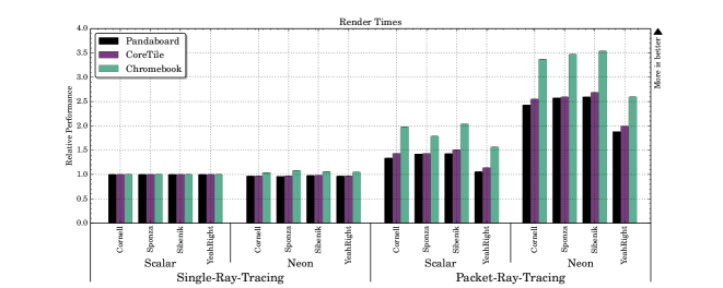
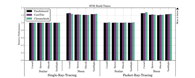
Using the ‘naïve’ ray tracer implementation, i.e. the scalar single-ray tracer as a reference we compute the relative improvement for each configuration and platform.
5.2 Scalability
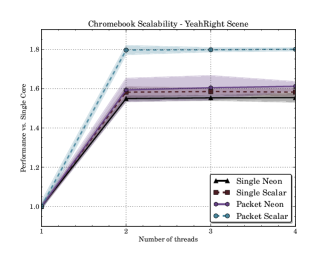
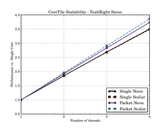
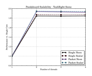
The scalability for each of the three platforms on the YeahRight scene is depicted in the plots in figure 5.5.
5.3 Power Performance
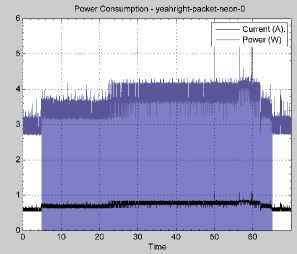
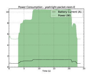
Many of the power results were created as plots, many of these are however very noisy and do not provide very detailed information of the actual energy consumption, thus we leave the majority of them out of the report. Some examples of this output are provided in figures 5.6a and 5.6b. Note however that the proper results are summarized in the tables below.
5.3.1 Baselines
The baseline energy consumption in idle mode for both the Pandaboard and the Chromebook are summarized in table 5.1.
| Platform | Energy Consumption |
|---|---|
| Pandaboard | W |
| Samsung Chromebook | W |
5.3.2 Energy Consumption - Pandaboard
Our estimate for the energy consumption for the whole application running in either single-ray- or packet-ray-tracing mode are summarized in table 5.2. The energy consumption relative to the scalar single-ray tracer can be seen in table 5.3.
| Scene | Single-Ray-Tracing | Packet-Ray-Tracing | |||
|---|---|---|---|---|---|
| Scalar | Neon | Scalar | Neon | ||
| Cornell | J | ||||
| Sponza | J | ||||
| Sibenik | J | ||||
| YeahRight | J | ||||
| Scene | Single-Ray-Tracing | Packet-Ray-Tracing | ||
|---|---|---|---|---|
| Scalar | Neon | Scalar | Neon | |
| Cornell | 1.00 | 1.27 | 1.23 | 2.44 |
| Sponza | 1.00 | 1.12 | 1.46 | 2.52 |
| Sibenik | 1.00 | 1.00 | 1.28 | 2.19 |
| YeahRight | 1.00 | 1.02 | 1.00 | 1.64 |
5.3.3 Energy Consumption - Chromebook
Estimates for the energy consumption for the whole application for the Chromebook are compiled in table 5.4 for both single-ray and packet-tracing modes. Likewise, the relative energy consumption is compiled in table 5.5.
| Scene | Single-Ray-Tracing | Packet-Ray-Tracing | |||
|---|---|---|---|---|---|
| Scalar | Neon | Scalar | Neon | ||
| Cornell | J | ||||
| Sponza | J | ||||
| Sibenik | J | ||||
| YeahRight | J | ||||
| Scene | Single-Ray-Tracing | Packet-Ray-Tracing | ||
|---|---|---|---|---|
| Scalar | Neon | Scalar | Neon | |
| Cornell | 1.00 | 1.08 | 1.46 | 2.10 |
| Sponza | 1.00 | 1.06 | 1.57 | 2.69 |
| Sibenik | 1.00 | 1.04 | 1.60 | 2.52 |
| YeahRight | 1.00 | 1.05 | 1.27 | 2.00 |
Chapter 6 Discussion
6.1 Runtime Performance
The most important result in this thesis is undoubtedly the rendertime but as seen among the results the scalability and BVH build time also contain interesting deviations that we will discuss to some extent.
6.1.1 Render Times
While it is possible to create a ray tracer that uses the SIMD vectors directly as the basic vector types, it is often not very effective in improving performance. This can easily be seen from our Neon accelerated single-ray tracer. In most cases the improvement is marginal at best and several times it even reduces the performance. Notably, the CoreTile and Pandaboard consistently perform a few percent worse, while the Chromebook perform a few percent better. This may be because the more powerful out-of-order execution in the A15 core can optimize the ‘bad’ code in hardware better than the A9 can. This kind of small performance dicrepancies are however very hard to find a reliable cause of and thus we will not look into it further.
It is possible that other ray tracer implementations or SIMD extensions can improve this but on the other hand, there are other ways to improve the performance already. This is shown with our packet tracer implementations: in almost all cases it can improve the performance by a factor between 2.0 - 3.5.
In raw rendering performance however, the Chromebook provides an additional 100% improvement over the CoreTile and Pandaboard. This is easily explained by the additional SIMD width of the A15 processor: The Cortex-A15 processor can compute the result of a 128-bit vector directly, while the A9 has to split up the computations in two intermediate 64-bit vectors instead.
6.1.2 BVH Build Time
During this project, we knew we needed an acceleration data structure to achieve respectable speeds for larger scenes. Due to the limited time however, our implementation of the BVH build algorithm is in fact mostly unoptimized.
Therefore it is quite surprising to see a 20-25% improvement in the build time when enabling the Neon architecture. Looking into it however, there is a major loop inside the build algorithm which constructs a single AABB to encompass a number of primitives. This algorithm loops over all primitives, gathering their individual bounding-boxes and includes them with element-wise min/max operations. In our system, this particular loop can be seen in listing 3.
There is no difference between the various configurations for this code, yet Neon accelerates it anyways thanks to the efficient min/max SIMD operations. Given time however, it should be possible to accelerate the BVH build algorithm considerably more than this.
6.1.3 Scalability
Theoretically the ray tracer should scale linearly with the number of available compute units. On our platforms, this seems very accurate from our result on the CoreTile Express, as seen in figure 5.5b. It still scales slightly worse than expected, with an increase of a factor of around 1.8-1.9 when doubling the number of threads on the CoreTile and Pandaboard, yet it is sufficiently close to the theoretical limit. For some reason, the Chromebook scales notably worse, only increasing the performance with around 60% when activating both cores. So far we have not found a reliable answer to why this happens but a qualified guess is that the memory-system bottlenecks the CPU. That is, the memory cannot provide the CPU with enough work to keep it busy.
Interestingly enough, the different configurations of the ray tracer scales slightly differently, with a clear edge towards packet-tracing. Yet, it is not enough to make any larger impact with so few cores available. With the advance of ARM server processors with a significantly larger amount of cores, such as the Cavium ThunderX ([6]) with up to 48 cores, this might play a larger role in the future.
6.2 Power Performance
Obtaining reliable power measurements are often difficult and this project was no exception. The methods we used ended up yielding consistent results, yet they could likely have been more efficiently implemented. It is also possible that other methods could have yielded better and more accurate results.
On the other hand, the methods we used were simple – in particular for the Chromebook, and could easily be repeated or integrated into a script.
6.2.1 Scalar versus Neon
As we saw in the runtime section, performance-wise, there is no point in implementing a single-ray tracer with Neon. Judging from the results in tables 5.2 – 5.5 however, Neon can apparently save more energy than runtime.
Still, while the runtime performance for the packet tracer improved with a factor of around 2.0 - 3.5, going from the single-ray tracer to the packet tracer, the power consumption did not scale as well. Still, it is not bad, the scaling is just reduced to around 1.6 - 2.5 for the Chromebook and 2.0 - 2.7 for the Pandaboard.
6.2.2 Pandaboard versus Chromebook
Often, the energy consumption follow the runtime rather closely, since the longer it takes to run an application, the more energy it must consume. However, as can be seen in the examples in figures 5.6a and 5.6b, the Chromebook consumes almost three times as much power in full load than in idle. compared to the Pandaboard, which barely doubles the power going from idle to full-load. If we also factor in the baseline for each of the platforms, the Pandaboard once again consumes far less than the Chromebook.
There are several possible reasons for this, most importantly the power consumption increases greatly with higher clock speeds, and the Chromebook runs at a 70% higher clock frequency than the Pandaboard. Furthermore, the Cortex-A15 is known to use considerably more power than the Cortex-A9 processor due to the different underlying hardware.
This does not necessarily mean that the Pandaboard is better than the Chromebook. It simply means that if we need to balance cost and power consumption against performance, the A9 will come out on top. On the other hand, if runtime performance is more important than the power consumption, the A15 might be a better match.
Chapter 7 Conclusions
During the course of this project we have created two different ray tracing implementations: A single-ray tracer and a packet tracer, each capable of running with or without Neon acceleration. This has shown us that the ARM Neon architecture is a very capable extension to the ARMv7 ISA and as we have shown in appendix B, it is functionally similar to the Intel SSE architecture. The most important discrepancy between them is the lack of full IEEE-754 floating point support in Neon, but in many applications, such as ray tracing, that is not important.
While it is currently slightly more difficult to develop for ARM platforms due to different architecture, it is rapidly getting easier as the demand increases and the development tools matures. At the same time the platforms become more readily available and more powerful. Performance-wise however, the Neon optimized packet ray tracer improved the rendering speed with around 300% compared to our reference implementation, matching our earlier hypothesis and the ones Wald presented in his thesis [33].
Among our platforms, the Samsung Chromebook with the Cortex-A15 performs around 100% better than the CoreTile Express and Pandaboard with their Cortex-A9 CPUs. On the other hand, the Chromebook consumes on average almost twice as much energy as the Pandaboard in the same configurations (See section 5.3). This simply means that they are optimized for different applications: If speed is required the A15 might be more suitable, otherwise the A9 might be sufficient.
7.1 Future Work
This project ended up generating a large amount of data, and a lot of it made it into this report. Ray tracing is however a huge subject and this thesis has barely scratched the surface. There are still many things that may be interesting to investigate further.
First and foremost, Whitted’s algorithm is just among the first of many ray tracing algorithms and it only provides the most basic lighting effects. It would be very interesting to see if packet tracing with Neon could improve the performance in a path tracer or photon mapper. In general, the coherency among the rays in a packet is lost after a couple of recursive bounces and after a long path of them, the rays will often travel in very different directions, greatly reducing the effectiveness of the packet tracing. Other algorithms such as the Instant Global Illumination algorithm [33, 32] can keep the coherency among the rays and still provide believable indirect illumination.
Another aspect that should be considered are various other acceleration data structures. In this project we only used a fairly unoptimized BVH implementation, in practice there might be other data structures that might be better suited for acceleration with Neon. In particular, Wald recommended Kd-Trees [33] while the Embree project often use a kind of optimized BVH structure. Which of these might benefit the most from the Neon architecture remains an open question.
Also, in order to gain further insight into the performance of the ray tracer, a much more thorough investigation should be done on the assembly level of the code. In particular, it may be of interest to implement a complete packet tracer in assembly as a reference.
Finally, ARM recently introduced heterogeneous computing into the mobile computing segment with their so called big.LITTLE technology. This particular technology pairs one or more power-efficient but low-speed CPU cores with larger more powerful ones in order to provide a better compromise between speed and power consumption. This system does however come in various configurations, and in one of them the operating system gets full access to all underlying cores and can schedule whatever it deems useful to them. It would be very interesting to see how such a platform would scale going from a single core to using all of them. In theory it should still scale piecewise linearly.
References
- [1] (1968) Some techniques for shading machine renderings of solids. In Proceedings of the April 30–May 2, 1968, Spring Joint Computer Conference, AFIPS ’68 (Spring), New York, NY, USA, pp. 37–45. External Links: Link, Document Cited by: §1.2.1.
- [2] (2013-11) ARM c language extensions. ARM Limited. Note: Release 1.1 Cited by: §B.1, §B.4, footnote 1.
- [3] The arm compiler. Note: Last accessed 2014-06-12. http://ds.arm.com/ Cited by: §B.1.
- [4] (2013) ARMv7-ar architecture reference manual. ARM Limited. Note: Issue C Cited by: §B.4, §2.1.1.
- [5] (2014) ARMv8-a architecture reference manual. ARM Limited. Note: Issue A.b Cited by: §B.4.
- [6] Cavium thunderx. Note: Last accessed 2014-07-24. http://www.cavium.com/ThunderX_ARM_Processors.html Cited by: §6.1.3.
- [7] (1984-01) Distributed ray tracing. SIGGRAPH Comput. Graph. 18 (3), pp. 137–145. External Links: ISSN 0097-8930, Link, Document Cited by: §1.2.1.
- [8] Intel intrinsics guide. Note: Last accessed 2014-06-12. https://software.intel.com/sites/landingpage/IntrinsicsGuide/ Cited by: §B.4.
- [9] (2012) Cortex-a9 neon media processing engine: technical reference manual. ARM Limited. Note: Revision r4p1 Cited by: 2nd item.
- [10] Eigen is a c++ template library for linear algebra: matrices, vectors, numerical solvers, and related algorithms.. Note: Last accessed 2014-06-09. http://eigen.tuxfamily.org/index.php?title=Main_Page Cited by: Chapter 2.
- [11] FFmpeg. Note: Last accessed 2014-06-09. http://www.ffmpeg.org/ Cited by: Chapter 2.
- [12] (1972-09) Some computer organizations and their effectiveness. IEEE Trans. Comput. 21 (9), pp. 948–960. External Links: ISSN 0018-9340, Link, Document Cited by: §1.2.2.
- [13] GCC - the gnu compiler collection. Note: Last accessed 2014-06-09. https://gcc.gnu.org/ Cited by: §B.1, §1.2.2, Chapter 2, §C.3, Packet Ray Tracing with the ARM NEON Architecture.
- [14] (2006) Computer architecture, fourth edition: a quantitative approach. Morgan Kaufmann Publishers Inc., San Francisco, CA, USA. External Links: ISBN 0123704901 Cited by: Appendix A.
- [15] (2012-02-28) ISO/iec 14882:2011 information technology — programming languages — c++. International Organization for Standardization. External Links: Link Cited by: §1.4, §2.1.1.
- [16] (2013) A walk through the cortex-a mobile roadmap. Note: Last accessed 2014-05-20. http://community.arm.com/groups/processors/blog/2013/11/19/a-walk-through-the-cortex-a-mobile-roadmap Cited by: §3.1.
- [17] (1986-08) The rendering equation. SIGGRAPH Comput. Graph. 20 (4), pp. 143–150. External Links: ISSN 0097-8930, Link, Document Cited by: §1.2.1.
- [18] (1995-03) The visual instruction set (vis) in ultrasparc. In Compcon ’95.’Technologies for the Information Superhighway’, Digest of Papers., pp. 462–469. External Links: Document, ISSN 1063-6390 Cited by: §1.2.2.
- [19] The llvm compiler infrastructure. Note: Last accessed 2014-06-09. https://llvm.org/ Cited by: §B.1, §1.2.2, Chapter 2, §C.3, Packet Ray Tracing with the ARM NEON Architecture.
- [20] Microsoft visual c++ compiler. Note: Last accessed 2014-06-12. http://msdn.microsoft.com/en-us/vstudio/hh386302.aspx Cited by: §B.1.
- [21] (2012) Dynamic memory allocation for over-aligned data. Note: Last accessed 2014-04-22. http://www.open-std.org/jtc1/sc22/wg21/docs/papers/2012/n3396.htm Cited by: footnote 2.
- [22] NEON. Note: Last accessed 2014-06-10. http://www.arm.com/products/processors/technologies/neon.php Cited by: §1.1.
- [23] Pandaboard, exynos 5, performance comparison.. Note: Last accessed 2014-06-16. http://openbenchmarking.org/result/1112277-AR-OMAPCORTE46,1211256-RA-ATOMCORTE12 Cited by: §1.3, Chapter 3, Chapter 4.
- [24] Pandaboard. Note: Last accessed 2014-06-09. http://pandaboard.org/ Cited by: §1.1.
- [25] (2010) Physically based rendering, second edition: from theory to implementation. 2nd edition, Morgan Kaufmann Publishers Inc., San Francisco, CA, USA. External Links: ISBN 0123750792, 9780123750792 Cited by: §1.2.1, §2.2.
- [26] Pandaboard, exynos 5, performance comparison.. Note: Last accessed 2014-06-16. http://www.phoronix.com/scan.php?page=article&item=pandaboard_es&num=1 Cited by: §1.3, Chapter 3.
- [27] Samsung chromebook 1. Note: Last accessed 2014-06-09. http://www.samsung.com/uk/consumer/pc-peripherals/chrome-devices/chrome-devices/XE303C12-A01UK Cited by: §1.1.
- [28] (2003) Realistic ray tracing. 2 edition, A. K. Peters, Ltd., Natick, MA, USA. External Links: ISBN 1568811985 Cited by: 2nd item.
- [29] FFMPEG armv7 vfpv3 vs neon. Note: Last accessed 2014-06-17. http://processors.wiki.ti.com/index.php/ARM_Multimedia_Users_Guide Cited by: Chapter 2.
- [30] (2013-04) Power efficiency of ray tracing. Master’s Thesis, Lund University, Faculty of Engineering. Cited by: §1.3.
- [31] (2014) User and reference guide for the intel c++ compiler 14.0. Intel Corporation. Note: Last accessed 2014-06-18. https://software.intel.com/en-us/compiler_14.0_ug_c Cited by: §B.1, §B.2, §1.2.2.
- [32] (2002) Interactive global illumination using fast ray tracing. In Proceedings of the 13th Eurographics Workshop on Rendering, EGRW ’02, Aire-la-Ville, Switzerland, Switzerland, pp. 15–24. External Links: ISBN 1-58113-534-3, Link Cited by: §7.1.
- [33] (2004) Realtime Ray Tracing and Interactive Global Illumination. Ph.D. Thesis, Computer Graphics Group, Saarland University. Cited by: §1.3, §1.4, §2.1, Chapter 2, Chapter 4, §7.1, §7.1, Chapter 7.
- [34] (1980-06) An improved illumination model for shaded display. Commun. ACM 23 (6), pp. 343–349. External Links: ISSN 0001-0782, Link, Document Cited by: §1.2.1, §2.2.1.
- [35] (2013) Embree ray tracing kernels for cpus and the xeon phi architecture. In ACM SIGGRAPH 2013 Talks, SIGGRAPH ’13, New York, NY, USA, pp. 44:1–44:1. External Links: ISBN 978-1-4503-2344-4, Link, Document Cited by: §1.4, Chapter 2.
Appendix A ARM CPU Architectures
The two main CPUs used during this project are the ARM Cortex-A15 and Cortex-A9. They were chosen since, at the time of writing, they are the two best performing ARM processors that are widely available in many developer and consumer products alike.
Design-wise however, the instruction pipeline of these processors are rather similar but differ significantly with the more modern but simpler and power efficient Cortex-A7, as can be seen in Figure A.1.
All of these chips are however developed with different intents: The A7 is supposed to have superior power efficiency, the A9 provides a compromise between energy consumption and speed, while the A15 is the most powerful one at the expense of energy consumption.
Some of the major architectural features of each of these processors are summarized below in table A.1. For a brief explanation of the various hardware features, please see the glossary in the back. Much more detailed explanations can be found in e.g. Patterson & Hennessy [14].
| Cortex-A7 | Cortex-A9 | Cortex-A15 | |
| ISA | ARMv7 | ARMv7 | ARMv7 |
| Processor type | Superscalar | Superscalar | Superscalar |
| Execution order | In-order | Out-of-order | Out-of-order |
| Pipeline length | 8-stage | 8-11-stages | 15-stage |
| Clock rates | 1.2 – 1.6 GHz | 0.8 – 2.0 GHz | 1.0 – 2.5 GHz |
| Multiprocessing | 1-4 SMP Cores | 1-4 SMP Cores | 1-4 SMP Cores |
| Branch Prediction | No | Yes | Yes |
| SIMD width | 64-bit | 64-bit | 128-bit |
Appendix B SSE versus NEON
Over the years many different SIMD technologies have been developed and today some of the more notable ones are Intel x86 SSE and ARM NEON. Both SSE and NEON are technologies intended to allow vector processing of up to 4 scalar values simultaneously, due to the underlying processor design however, they have evolved quite differently. In this appendix we will briefly describe how these hardware technologies can be used in high-level programming languages such as C and C++ using so-called compiler Intrinsics.
We will however mostly limit the comparison to versions 1-4.2 of SSE, since afterwards Intel introduced the so called Advanced Vector Extensions, which doubled the vector widths to 256-bits. Since Neon is still only 128-bit, we will leave a comparison of these newer intrinsics for a potential future comparison
B.1 Compiler Support
The first thing that must be noted regarding compiler intrinsics: As the name suggest, they are internal to the compiler, and may not be portable. The intrinsics in both SSE and Neon are however well defined, with official naming schemes by Intel and ARM respectively, so compiler implementation of them should be consistent.
Officially, the LLVM [19], GCC [13] and The ARM Compiler [3] support the same Neon intrinsics, as they are defined by ARM C Language Extensions [2].
SSE has been around for far longer; it is also supported in LLVM and GCC, and in addition, it is supported in the Microsoft Visual C++ Compiler [20] and the Intel C++ Compiler [31].
Activating the SIMD intrinsics differs between the compilers and SIMD architecture however, most of them require a specific command-line flag to be activated during compilation. Table B.1 show some examples of compiling a simple test file with either Neon or SSE intrinsics.
| Compilers | SIMD | Command-line |
|---|---|---|
| MSVC | SSE | cl /arch:SSE /c /FA test.c |
| ICC | SSE | icc -msse test.c -o test.c |
| GCC | SSE | gcc -msse test.c -o test.c |
| Clang | SSE | clang -msse test.c -o test.c |
| ARMCC | NEON | armcc -mfpu=neon test.c -o test.c |
| GCC | NEON | gcc -mfpu=neon test.c -o test.c |
| Clang | NEON | clang -mfpu=neon test.c -o test.c |
B.2 Version Fragmentation
There has been many SIMD extensions added to the x86 ISA over the years. The MMX where the first one which added support for 64-bit wide SIMD vectors, with either 8x8, 16x4, 32x2 or 64x1 integer vectors. The MMX extension did however have several major architectural flaws: It had to share registers with the stack-based FPU and required user assisted register-flushes going between FPU and MMX processing [31], making it difficult to use and error prone. These shortcomings were rectified with the introduction of SSE, which introduced dedicated registers for all vector operations.
Over the years, additional versions of SSE were created, adding more intrinsics and versatility with each successive version. This fragmentation does however make it difficult for software vendors; they have to maintain separate code paths for new and old intrinsics if the code is going to be portable to older x86 platforms that do not support all SSE versions.
For ARM it is somewhat easier since there are currently only a few versions of Neon available. It does however seem like it might change with the introduction of the ARMv8 ISA which adds several new intrinsics that cannot be used on ARMv7 products.
B.3 SIMD Data Types
The compiler extensions provide several new base data types for working with the SIMD vectors. Neon and SSE uses these types very differently however: SSE have the same base type for several kinds of different vectors, while Neon have dedicated types for each different kind of vector. The SSE data types are described in greater detail in section B.3.1, and the Neon types are described in section B.3.2.
B.3.1 SSE Types
The SSE data types typically represent the bit-sizes of the Intel SIMD registers. Several kinds of vectors are however shared between a single data type, as described in table B.2:
| Name | Description |
|---|---|
| __64 | Vector type with either 8 8-bit, 4 16-bit or 2 32-bit signed or unsigned integers. |
| __int64 | Signed or unsigned integer type with 64-bits. |
| __128 | Floating point type with four 32-bit floating point values. |
| __128i | Vector type with either 16 8-bit, 8 16-bit, 4 32-bit, or 2 64-bit signed or unsigned integer types. |
| __128d | Floating point type with two 64-bit floating point values. |
B.3.2 Neon Types
Neon provides new base types for each possible vector type and follows the predictable naming scheme as seen below:
<type><size>x<number of lanes>_t
All of the possible data types are listed in table B.3.
| 64-bit types | 128-bit types | |||||
|---|---|---|---|---|---|---|
| int8x8_t | uint32x2_t | uint8x8_t | int8x16_t | uint32x4_t | uint8x16_t | |
| int16x4_t | uint64x1_t | uint16x4_t | int16x8_t | uint64x2_t | poly8x16_t | |
| int32x2_t | float16x4_t111The half precision float is only a data type. There are no operations that can be performed on it [2]. | poly8x8_t | int32x4_t | float16x8_t | uint16x8_t | |
| int64x1_t | float32x2_t | poly16x4_t | int64x2_t | float32x4_t | poly16x8_t | |
B.3.3 Comparing the Data Types
Comparing just the available vector types for the SIMD extensions, we can see some distinct disadvantages to both approaches:
-
•
Neon does not have any support for vectors of 64-bit floating point types.
-
•
For SSE, integer vectors share base types which requires the user to keep track of the actual type inside the vector by herself. With Neon, some of this work can be offloaded to the compiler instead. Creating typedefs might make the type management easier with SSE, but that can lead to namespace issues instead.
-
•
Neon has the binary polynomial (poly) data-types and SSE has no direct equivalent to these. The behaviour can however be simulated with a mix of other intrinsics.
B.4 The Intrinsics
Most of the intrinsics available for both technologies follow a set of naming schemes to make them easier to remember. For SSE, most intrinsics use the following naming convention.
_mm_<intrin-op>_<sse-type-suffix>
Neon on the other hand, uses a different naming scheme:
<intrin-op><flags>_<neon-type-suffix>
For a more detailed explanation of the each item, see the following table:
| Item | Description |
|---|---|
| intrin-op | Special op-code name for the intended operation. E.g., add to add two vectors, or and to perform bit-wise AND on two vectors. Note however that SSE and Neon frequently use different names for the same operation. |
| sse-type-suffix | Suffix used by SSE to define the actual data-type inside the available data-types (Table B.2). The first one or two letters determines whether the data is packed (p), extended packed (ep), or scalar (s). If the types are any kind of a packed type, we operate on all elements. If it is scalar, we only operate on the first one. The remaining letters denote the data type of the vector content, see table B.4 to see which ones are available. |
| neon-type-suffix | Suffix used by Neon to determine which data type we will operate on. The suffix available can be seen in table B.4. |
| flags | This Neon specific flag determines whether we will operate on a 128-bit vector or a 64-bit one. This flag can also specify extra operations such as double the content, or widen the size bit-size of the element afterwards. |
| Vector Type | SSE | Neon |
|---|---|---|
| Signed integer | i<#bits> | s<#bits> |
| Unsigned integer | u<#bits> | u<#bits> |
| Float | s | f32 |
| Double | d | — |
Both SIMD extensions provide most of the common arithmetic operations one would expect for working with vectors, such as element-wise addition, subtraction and multiplication. A complete reference over all x86 intrinsics available, if implemented by the compiler can be found in the Intel Intrinsics Guide [8]. For the Neon intrinsics, refer to the ARM Architecture Manuals [4, 5] or ARM C Language Extensions [2].
There are several discrepancies between the different extensions and their intrinsics, in particularly regarding the integer intrinsics. The full list of discrepancies would however be far too long and not provide much insight; instead we will only look at some of the more interesting ones in the following sections.
B.4.1 Vector Permutations
One of the greater strengths in the SSE is the fast shuffle instruction: _mm_shuffle. This operation can then quickly create an arbitrary combination of elements from the given vector. It does however work slightly differently for floating point and integer types: The float variant takes two (possibly different) vectors, and blends the content based on an bit-mask. The integer variants only accept a single vector. The whole operation is explained with pseudocode and illustration in figure B.1.
⬇ _mm_shuffle(vec a, vec b, int imm) { SELECT4(src, control) { switch(control[1:0]) { 0: tmp[31:0] := src[31:0] 1: tmp[31:0] := src[63:32] 2: tmp[31:0] := src[95:64] 3: tmp[31:0] := src[127:96] } return tmp[31:0] } dst[ 31: 0] := SELECT4(a[127:0], imm[1:0]) dst[ 63:32] := SELECT4(a[127:0], imm[3:2]) dst[ 95:64] := SELECT4(b[127:0], imm[5:4]) dst[127:96] := SELECT4(b[127:0], imm[7:6]) }
Neon has no equivalent to these intrinsics. Instead it provides a variety of instructions to rearrange some of the contents e.g., the vrevq and vextq reverses and circularly rotates the contents respectively. Combining these and other such intrinsics can always yield the wanted combination, but there is no intrinsic that can do an arbitrary shuffle with a single instruction.
B.4.2 Arithmetic Intrinsics
Most basic arithmetic intrinsics are practically equivalent among the SIMD architectures. SSE does however provide some more exotic operations. E.g., it has dedicated instructions for computing the square root, division and dot-product.
Meanwhile Neon has some dedicated instructions to partially compute the next iteration step for Newton-Raphson approximation for the reciprocal and reciprocal square root. Neon also has a plethora of operations for extracting a single element from a vector to e.g., multiply all elements of another vector with. Finally, some Neon implementations also have a wide variety of fused multiply accumulate instructions. These operations are however available in the more recent x86 extensions: AVX2 and XOP for Intel and AMD respectively.
B.4.3 Load/Store Intrinsics
Neon and SSE both provide intrinsics to load/store a vector from a (possibly) unaligned memory location. They also both provide operations to load a value from memory, and ‘splat’ it across the vector. In Intel terminology, this is usually called a broadcast operation, while ARM typically call it duplicating operation.
Neon does however also provide a large amount of multi-register load and store operations, that can optionally interleave/deinterleave the contents into the registers. This makes it possible to rapidly separate e.g. colors into separate registers and operate on them directly. SSE has no direct equivalent but can often use the inexpensive shuffle operation to separate the values after a load instead. Although this is often more expensive than having it done directly in the memory pipeline.
B.4.4 Miscellaneous Intrinsics
Another interesting intrinsic in SSE is the _mm_movemask instruction. Given a float vector it can quickly extract the sign bits for each individual element and reduce it to a 32-bit integer bit-mask from these. Since comparison operations create vector bit-masks, it is possible to use this operations to quickly perform binary decisions based on the returned mask. E.g., one can query the returned bit mask for if all, any or none of the elements in a vector are set.
For some applications, such as ray tracing, this is very valuable since we will often make a decision based on if any, or none of the contents in a vector comparison is true. Neon has no direct equivalent to this operation, and to simulate it, costly vector- to regular-registers has to be performed.
Other than the above masking intrinsic, SSE also provide many types of string comparison instructions, such as the _mm_cmpistra. These are however very limited to small strings but can in series provide reasonable acceleration for longer strings as well.
B.5 Assorted Notes
Below is a small assortment of notes regarding some limitations and pitfalls with the various architectures.
-
•
Neon floating point vectors are not fully compliant with the IEEE-754 standard:
-
–
Denormals are flushed to zero.
-
–
Rounding is fixed to round-to-nearest with the exception of the explicit rounding intrinsics.
-
–
-
•
The scalar floating-point instructions are completely separated from the Neon pipeline and mixing regular floating point- and Neon-instructions will trigger expensive pipeline-flushes [9].
-
•
Neon does not support double Precision floating point operations.
-
•
In SSE, vectors with just 2 32-bit elements can use the legacy MMX operations but those can be error prone to use. Often it is possible to utilize the SSE intrinsics instead but then two elements might be wasted inside the SSE registers.
B.6 Conclusions
As can be seen above, for modern processors with at least SSE 4.2, Neon and SSE are pretty much equivalent in most regards. There are however notable discrepancies. Neon i.e., has a greater plethora of load/store operations, but SSE can quickly shuffle the loaded vectors around instead. A potentially larger pitfall is the lack of IEEE-754 compliance in Neon, which might make it less useful for scientific computations, but for media acceleration it makes almost no difference.
On the horizon however, Intel have already developed the so called AVX extension, working with 256-bit vectors fragmented into various different versions similar to how SSE is fragmented. Furthermore, the Many Integrated Core or MIC architecture, marketed as Xeon Phi, which provide an even wider SIMD architecture, with vectors up to 512-bits.
Meanwhile, ARM has developed the ARMv8 ISA which adds several improvements to the existing Neon architecture such as new reduction intrinsics, full IEEE-754 floating point support and double precision floating point data types. The vector-width does not seem to increase for a while yet however.
Appendix C Additional Data
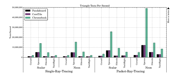
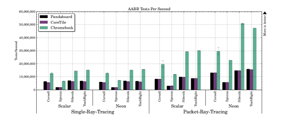
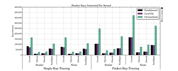
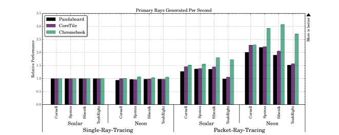
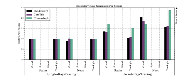
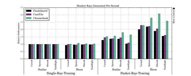
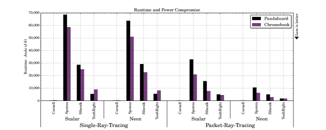
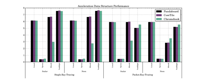
This chapter contains some additional data gathered during the course of the project but is not thouroughly analysed or discussed. In particular, the number of AABB and triangle tests per second as well as the number of primary, secondary and shadow rays generated per second are compiled here. In addition, some derived plots such as a measurement of power efficiency and acceleration data structure utilization can be found here.
C.1 Intersection Tests
This section contains the number of intersection tests executed per second as well as the results relative to the scalar single-ray tracer.
C.2 Rays Generated Per Second
C.3 Derived Computations
This section contains some derived results such as a measurement of the power efficiency and acceleration data structure utilization.
Glossary
- AABB
- An Axis Aligned Bound Box (AABB) is an object that is intended to wrap one or more primitives inside very basic three dimensional structure that is aligned with each of the primary axes
- Alignment
- The way memory is arranged and accessed. E.g., when an address is a multiple of 4, it is aligned to 4-byte boundary
- ARM
- A family of instruction set architectures based on the RISC architecture developed by the British company ARM Holdings
- AVX
- Advanced Vector Extensions
- Branch Prediction
- A hardware feature which tries to guess which branch will be taken during execution, which can reduce the number of costly pipeline flushes
- BSP
- Binary Space Partitioning
- BVH
- Bounding Volume Hierarchy
- CPU
- Central Processing Unit
- FPU
- A Floating Point Unit (FPU) is a hardware component dedicated to floating point, i.e., ‘decimal’ arithmetic
- GCC
- The GNU Compiler Collection [13]
- GPU
- Graphics Processing Unit
- In-Order Processor
- A processor that processes one instruction after another in the order they are received. Contrasts with out-of-order processors
- Intrinsics
- A term referring to a compiler specific, or non-standardized extension that give users access to low-level, processor specific instructions in high-level programming languages, such as C or C++. E.g. SIMD intrinsics allows us to use SIMD instructions directly without writing assembly code
- ISA
- An Instruction Set Architecture (ISA) describes all available instructions available for application and system programmers for a given platform
- LLVM/Clang
- The Low Level Virtual Machine (LLVM) is a compiler infrastructure project. Clang is the C/C++/C# frontend of LLVM. LLVM/Clang is often used interchangeably to refer to the whole compiler infrastructure [19]
- Mesh
- A collection of triangles, structured in some way
- NEON
- Marketing name for the SIMD extensions available to ARMv7 processors. Officially, it is known as the Advanced SIMD Extension
- Out-of-Order Processor
- A processor that can rearrange instructions based on dependencies at the register level in order to improve the instruction level parallelism. These processors can potentially increase the instruction throughput of the processor but often require larger areas of silicon and consume more power than an in-order equivalent processor
- Primitive
- Any basic object that can be visualized with computer graphics algorithms. The most commonly used primitive is the triangle
- Shade
- A colloquial term for applying colors, effects or textures to objects, altering their appearance
- SIMD
- Single Instruction Multiple Data (SIMD) is a part of Flynn’s taxonomy where a single instruction can work on multiple individual pieces of data
- SMP
- Abbreviation for Symmetric Multiprocessing, a hardware feature that allows a number of physical processor cores to share the same main memory
- SoC
- A System on Chip (SoC) is a term used to describe a complete hardware platform, typically for embedded systems
- SSE
- Streaming SIMD Extensions
- Superscalar Processor
- A processor that can forward more than single instruction along the processor pipeline at once
- x86
- A family of backward compatible instruction set architectures, primarily of CISC design